Quick Guide

Here you can find a short overview of all package modules as well as some main applications with pyrexMD. Most functions are workflow-orientated so that you can perform complex tasks (e.g. system setup, specific analyses, etc.) within a few commands. This guide is kept very short because most commands have an obvious ‘core’ functionality. All code snippets in this quick guide are taken from the Jupyter notebooks within the example folder, which you can use to run and test the package on your local machine.

Important

Most analysis functions for calculating useful quantities such as RMSDs, Q values, contact distances, etc., can generate figures in the same step if the keyword argument plot=True is passed. Please refer to the API docs in order to get the most out of plot-generating functions, as they usually allow many valid keyword arguments.

Module Overview

pyrexMD.core: Contains functions enabling interactive analyses. Its main parts are the iPlayer and iPlot classes, which allow the use of a trajectory viewer or a dynamic linking of the trajectory viewer and any 2D graph.
pyrexMD.gmx: Contains modified GromacsWrapper functions for streamlining the interaction with GROMACS for system setups etc.
pyrexMD.rex: Contains functions related to (contact-guided) Replica Exchange Molecular Dynamics, mainly for automating and speeding up the simulation setup.
pyrexMD.topology: Contains functions for modifying universe topologies, e.g., align atoms/residues of two universes, get matching selection strings, include bias contacts.
pyrexMD.analysis.analyze: Contains various functions for basic trajectory analyses, e.g., calculating RMSDs, distances, etc.
pyrexMD.analysis.cluster: Contains functions for decoy clustering and post-REX clustering analyses.
pyrexMD.analysis.contacts: Contains functions for native-contact and bias-contact analyses.
pyrexMD.analysis.dihedrals: Contains functions for dihedral-angle analyses.
pyrexMD.analysis.gdt: Contains functions for global distance test (GDT) analyses.
pyrexMD.misc: Consists of pyrexMD.misc.classes, pyrexMD.misc.func, and pyrexMD.misc.plot. This sub-package is a collection of miscellaneous and frequently used functions and classes. These functions may contain modified versions of small existing functions to extend their default behavior in order to streamline pyrexMD.

Application Overview

Setup of Normal MD Simulation

Using GROMACS in pyrexMD is very similar to the known command-line syntax. Commands such as

gmx function -p parameter

simply become:

gmx.function(p=parameter)

Additionally to the expected GROMACS behavior, each gmx module function creates by default a unique log file with a meaningful name which is stored in the logs folder.

The code example below shows a complete setup of a normal MD simulation.

import pyrexMD.gmx as gmx
import pyrexMD.misc as misc

# create ref pdb:
pdb = "path/to/pdb"
ref = gmx.get_ref_structure(pdb, ff='amber99sb-ildn', water='tip3p', ignh=True)

# generate topology & box
gmx.pdb2gmx(f=ref, o="protein.gro", ff='amber99sb-ildn', water='tip3p', ignh=True)
gmx.editconf(f="protein.gro", o="box.gro", d=2.0, c=True, bt="cubic")

# copy mdp files (ions.mdp, min.mdp, nvt.mdp, npt.mdp, md.mdp) into working directory
misc.cp("path/to/mdp/files", ".")

# generate solvent & ions
gmx.solvate(cp="box.gro", o="solvent.gro")
gmx.grompp(f="ions.mdp", o="ions.tpr",c="solvent.gro")
gmx.genion(s="ions.tpr", o="ions.gro", neutral=True, input="SOL")

# minimize
gmx.grompp(f="min.mdp", o="min.tpr", c="ions.gro")
gmx.mdrun(deffnm="min")

# NVT equilibration
gmx.grompp(f="nvt.mdp", o="nvt.tpr", c="min.gro", r="min.gro")
gmx.mdrun(deffnm="nvt")

# NPT equilibration
gmx.grompp(f="npt.mdp", o="npt.tpr", c="nvt.gro", r="nvt.gro", t="nvt.cpt")
gmx.mdrun(deffnm="npt")

# MD run
gmx.grompp(f="md.mdp", o="traj.tpr", c="npt.gro", t="npt.cpt")
gmx.mdrun(deffn="traj")

Setup of Contact-Guided REX MD Simulation

The code example below shows a complete setup of a contact-guided REX MD simulation using different starting conformations (“decoys”) for each individual replica. It automates many system-specific and arduous tasks to eliminate possible application errors, such as mismatching system sizes across replicas, incorrect mapping of bias contacts, etc.

import pyrexMD.misc as misc
import pyrexMD.rex as rex
import pyrexMD.topology as top

decoy_dir = "path/to/decoy/directory"

# create rex_i directories and assign decoys
rex.assign_best_decoys(decoy_dir)
rex_dirs = rex.get_REX_DIRS()

# check for consistent topology
rex.check_REX_PDBS(decoy_dir)

# copy mdp files (ions.mdp, min.mdp, nvt.mdp, npt.mdp, rex.mdp) into working directory
misc.cp("path/to/mdp/files", ".")

# get parameters for fixed box size and solvent molecules
boxsize, maxsol = rex.WF_get_system_parameters(wdir="./rex_0_get_system_parameters/")

# create systems for each replica
rex.WF_REX_setup(rex_dirs=rex_dirs, boxsize=boxsize, maxsol=maxsol)

# minimize
rex.WF_REX_setup_energy_minimization(rex_dirs=rex_dirs, nsteps=10, verbose=False)

# add bias contacts (RES pairs defined in DCA_fin)
top.DCA_res2atom_mapping(ref_pdb=<ref_pdb>, DCA_fin=<file_path>, n_DCA=50, usecols=(0,1))
top.DCA_modify_topology(top_fin="topol.top", DCA_used_fin=<file_path> , k=10, save_as="topol_mod.top")

# prepare temperature distribution
rex.prep_REX_temps(T_0=280, n_REX=len(rex_dirs), k=0.006)

# create mdp and tpr files
rex.prep_REX_mdp(main_dir="./", n_REX=len(rex_dirs))
rex.prep_REX_tpr(main_dir="./", n_REX=len(rex_dirs))

# next: upload REX MD run files on HPC and execute production run

Interactive Plots

pyrexMD can generate interactive plots by linking a 2D graph to the trajectory viewer of a specific universe. It allows to quickly inspect conformations at specific values by interacting with the graph itself (e.g. via ctrl-click). In this way, additional valuable information becomes accessible through the trajectory viewer.

import MDAnalysis as mda
import pyrexMD.misc as misc
import pyrexMD.core as core
import pyrexMD.topology as top
import pyrexMD.analysis.analyze as ana

# set up universe
ref = mda.Universe(<pdb_file>)
mobile = mda.Universe(<tpr_file>, <xtc_file>)

# calculate RMSD
FRAMES, TIME, RMSD = ana.get_RMSD(mobile, ref=ref, sel1="protein", sel2="protein")

# create interactive plot
IP = core.iPlot(mobile, xdata=TIME, ydata=RMSD, ylabel=r"RMSD (A)")
IP()

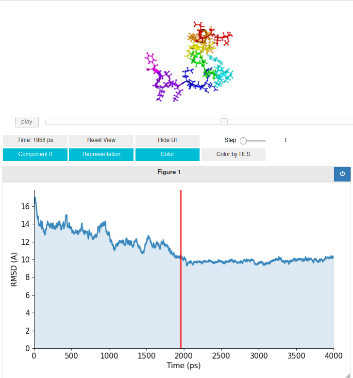
In this example, the interactive plot links the RMSD time evolution graph to the flexible trajectory.

Contact and Bias Analyses

REX is a very powerful and versatile sampling method. It improves sampling by running many replicas in parallel over a wide temperature range and allows switches of replicas between different temperatures while maintaining thermodynamic ensembles. By integrating (theoretical, experimental, or mixed) bias contacts via bias potentials, one can narrow down the search space and guide the simulations towards specific conformations. This speeds up the process and lowers the computational costs. pyrexMD covers many different forms of contact and bias analyses.

import MDAnalysis as mda
import pyrexMD.misc as misc
import pyrexMD.topology as top
import pyrexMD.analysis.analyze as ana
import pyrexMD.analysis.contacts as con

# set up universes
folded = mda.Universe(<pdb_file_folded>)
unfolded = mda.Universe(<pdb_file_unfolded>)
mobile = mda.Universe(<tpr_file>, <xtc_file>)
top.norm_universe([folded, unfolded, mobile])

# check True Positive Rate (TPR) of predicted bias contacts
con.plot_DCA_TPR(folded, DCA_fin=<path_to_predicted_contacts>, n_DCA=80, d_cutoff=8.0)

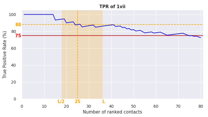
The figure shows:

blue line: TPR for number of ranked contacts
red line: 75% threshold (TPR of used contacts should be above approx. 75% for contact-guided REX MD, see https://doi.org/10.1371/journal.pone.0242072)
orange lines: suggested/guessed optimum number of contacts and the corresponding TPR
orange region: suggested region of interest between L/2 and L contacts (L = biomolecular sequence length)

# calculate QValue for realized bias contacts
bias_contacts = misc.read_file(<path_to_used_contacts>, usecols=(0,1))
FRAMES, QBIAS, CM = con.get_QBias(mobile, bc=bias_contacts)

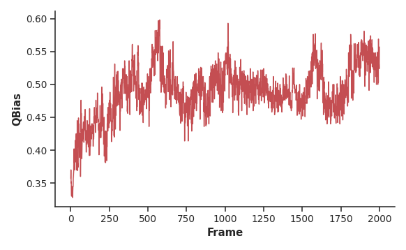
pyrexMD distinguishes mainly between two types of Q values, i.e., QNative (fraction of native contacts) and QBias (fraction of realized bias contacts). Both types can be used for structure analyses; however, when simulating unknown target structures QNative becomes inaccessible due to the missing reference structure.

# create log files with native contacts at different conformations
con.get_Native_Contacts(unfolded, sel="protein", save_as="unfolded_contacts.txt")
con.get_Native_Contacts(folded, sel="protein", save_as="folded_contacts.txt")

# check which contacts formed or broke up via ContactMap
fig, ax = con.plot_Contact_Map(folded, DCA_fin="unfolded_contacts.txt", sel="protein")

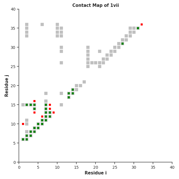
pyrexMD‘s Contact Maps show native contacts in grey and check whether bias contacts are native (green) or non-native (red). This functionality can be used to either compare and validate the used bias contacts or compare two structures and show the newly formed and broken contacts in green and red, respectively.

# check native contact distances via ContactMap
NC, NC_dist, DM = con.get_NC_distances(folded, folded)
con.plot_Contact_Map_Distances(folded, NC=NC, NC_dist=NC_dist, sel="protein")

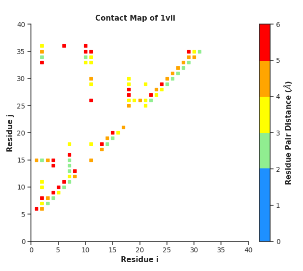
Additionally, it is possible to analyze native contact distances within a contact map plot. This can be used to deduce how strong/important the invidiual contacts are regards to structure stability.

GDT and LA Analyses

The so-called global distance test (GDT) is a method for structure evaluation similar to the root-mean-square deviation (RMSD). However, RMSD is a suboptimal measure of structural similarity as it strongly correlates with the largest displacement between mobile and target structure. If the mobile structure globally fits the target to a large extent and only one small segment is misaligned locally, the RMSD becomes disproportionately large. For the GDT, the mobile structure is first aligned to the target structure analogously to an RMSD analysis. To estimate how similar the two structures are, the displacement of each residual Cα atom is calculated and compared to various cutoffs. In a last step, percentages of residues with displacements below a considered threshold are used to calculate scores. The two most common scores are the total score (TS),

\[GDT_{\rm{TS}} = \frac{1}{4} (P_1 + P_2 + P_4 + P_8),\]

and the high-accuracy (HA) score,

\[GDT_{\rm{TS}} = \frac{1}{4} (P_{0.5} + P_1 + P_2 + P_4),\]

where \(P_x\) denote the percentage of residues with displacements below a distance cutoff of x Å.

import MDAnalysis as mda
import pyrexMD.misc as misc
import pyrexMD.core as core
import pyrexMD.topology as top
import pyrexMD.analysis.analyze as ana
import pyrexMD.analysis.gdt as gdt

# set up universes
ref = mda.Universe("<pdb_file>")
mobile = mda.Universe("<tpr_file>", "<xtc_file>")
top.norm_and_align_universe(mobile, ref)

# perform GDT (Global Distance Test)
GDT = gdt.GDT(mobile, ref)
GDT_percent, GDT_resids, GDT_cutoff, RMSD, FRAME = GDT

# calculate GDT scores
GDT_TS = gdt.get_GDT_TS(GDT_percent)
GDT_HA = gdt.get_GDT_HA(GDT_percent)

# rank scores
SCORES = gdt.GDT_rank_scores(GDT_percent, ranking_order="GDT_TS", verbose=False)
GDT_TS_ranked, GDT_HA_ranked, GDT_ndx_ranked = SCORES

# generate plots
ana.PLOT(xdata=frames, ydata=GDT_TS, xlabel="Frame", ylabel="GDT TS")
ana.plot_hist(GDT_TS, n_bins=20, xlabel="GDT TS", ylabel="Counts")

# Local Accuracy plot
gdt.plot_LA(mobile, ref, GDT_TS_ranked, GDT_HA_ranked, GDT_ndx_ranked)

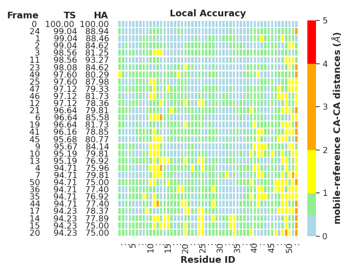
The local accuracy (LA) plot clearly shows how good each model part is refined compared to a reference structure. It is possible to show/hide each of the information columns (FRAME, TS and HA) individually.

Cluster Analyses

REX MD simulations generate large amounts of data. Depending on the project goal, filtering and clustering of structural ensembles will be necessary.

import pyrexMD.misc as misc
import pyrexMD.analysis.cluster as clu

# load data of pre-filtered frames
QDATA = misc.pickle_load("./data/QDATA.pickle")
RMSD = misc.pickle_load("./data/RMSD.pickle")
GDT_TS = misc.pickle_load("./data/GDT_TS.pickle")
score_file = "./data/energies.log"
ENERGY = misc.read_file(score_file, usecols=1, skiprows=1)
DM = clu.read_h5("./data/DM.h5")

# apply TSNE for dimension reduction
tsne = clu.apply_TSNE(DM, n_components=2, perplexity=50)

### apply KMeans on TSNE-transformed data (two variants with low and high cluster number)
# note: here we set the high number only to 20 because our sample is small with only 500 frames
cluster10 = clu.apply_KMEANS(tsne, n_clusters=10)
cluster20 = clu.apply_KMEANS(tsne, n_clusters=20)


### plot cluster data
# here: TSNE-transformed data with n_clusters = 20
# also: plot cluster centers with different colors
#     - red dot: n10 centers
#     - black dot: n20 centers
clu.plot_cluster_data(cluster20, tsne)
clu.plot_cluster_center(cluster10, marker="o", color="red", ms=20)
clu.plot_cluster_center(cluster20, marker="o", color="black")

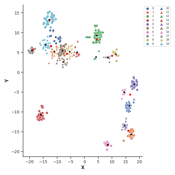
The example code above applies t-distributed stochastic neighbor embedding (TSNE) for dimension reduction of distance matrices (DM). Afterwards, a ‘fine’ and ‘coarse’ KMeans clustering is performed with 10 and 20 cluster centers, respectively.

It is possible to link both scores and structure accuracy to clusters, which can be used to select or compare the individual cluster ensembles, e.g. with

### map scores (energies) and accuracy (GDT, RMSD) to clusters
cluster10_scores = clu.map_cluster_scores(cluster_data=cluster10, score_data=score_file)
cluster10_accuracy = clu.map_cluster_accuracy(cluster_data=cluster10, GDT=GDT_TS, RMSD=RMSD)
cluster20_scores = clu.map_cluster_scores(cluster_data=cluster20, score_data=score_file)
cluster20_accuracy = clu.map_cluster_accuracy(cluster_data=cluster20, GDT=GDT_TS, RMSD=RMSD)

### print table with cluster scores stats
clu.WF_print_cluster_scores(cluster_data=cluster10, cluster_scores=cluster10_scores)
clu.WF_print_cluster_scores(cluster_data=cluster20, cluster_scores=cluster20_scores)

This prints a summary of the cluster scores (which can also be saved to a log file if the save_as value is set).

cluster n10 scores (ranked by Emean)

ndx  size  compact | Emean    Estd    Emin      Emax      DELTA
 77     6.695 |-230.652  6.975  -246.249  -211.738  -7.67
 61      5.78 |-226.274  8.08   -241.86   -209.002  -3.292
 43     3.098 |-225.174  7.679  -242.951  -206.42   -2.192
 52     2.807 |-224.486  7.592  -240.913  -202.431  -1.504
 41     9.439 |-223.741  17.481 -249.136  -190.634  -0.759
 53     3.441 |-223.03   6.056  -237.002  -209.372  -0.048
 25     2.172 |-220.319  7.431  -231.002  -203.796   2.663
 80     9.121 |-216.962  7.09   -235.155  -200.969   6.02
 25     0.798 |-214.371  6.688  -228.33   -201.657   8.611
 43      1.91 |-194.022  2.585  -198.461  -190.412   28.96
-------------------------------------------------------------------
cluster n20 scores (ranked by Emean)

ndx  size  compact | Emean    Estd    Emin      Emax      DELTA
 12     1.115 |-236.354  12.82  -249.136  -201.079  -13.372
 22     2.137 |-231.452  5.878  -243.144  -219.911  -8.47
 18      1.76 |-231.239  5.605  -246.249  -220.788  -8.257
 14     0.497 |-230.679  11.003 -246.674  -208.399  -7.697
 20      2.16 |-230.552  5.368  -242.131  -219.766  -7.57
 31     1.638 |-229.789  8.104  -241.151  -211.738  -6.807
 15     1.398 |-228.603  6.845  -241.86   -212.383  -5.621
 43     3.098 |-225.174  7.679  -242.951  -206.42   -2.192
 44     2.291 |-224.619  7.811  -240.913  -202.431  -1.637
 8      0.384 |-223.752  6.2    -231.774  -211.164  -0.77
 22     0.687 |-223.718  5.461  -236.263  -217.044  -0.736
 15     0.448 |-222.686  6.776  -230.6    -205.661   0.296
 31     1.334 |-222.541  6.4    -237.002  -209.372   0.441
 36      2.35 |-222.276  8.934  -238.79   -203.796   0.706
 21     0.526 |-221.485  7.025  -231.002  -207.53    1.497
 33     1.409 |-217.024  6.648  -235.155  -204.817   5.958
 25     0.798 |-214.371  6.688  -228.33   -201.657   8.611
 32     0.946 |-214.215  5.974  -231.045  -200.969   8.767
 15     0.894 |-207.389  12.28  -235.212  -190.634   15.593
 43      1.91 |-194.022  2.585  -198.461  -190.412   28.96

Analogously, the cluster accuracy can be displayed with

### print table with cluster accuracy stats
clu.WF_print_cluster_accuracy(cluster_data=cluster10, cluster_accuracy=cluster10_accuracy)
clu.WF_print_cluster_accuracy(cluster_data=cluster20, cluster_accuracy=cluster20_accuracy)

and results in

cluster n10 accuracy (ranked by GDT mean)

                   | GDT     GDT    GDT     GDT    | RMSD   RMSD   RMSD   RMSD
ndx  size  compact | mean    std    min     max    | mean   std    min    max
  52    2.807 | 77.296  1.815  73.81   80.953 | 2.555  0.154  2.182  3.076
  77    6.695 | 77.003  2.451  63.69   82.44  | 2.804  0.096  2.62   3.154
  61     5.78 | 75.943  2.325  71.728  82.142 | 2.85   0.096  2.567  3.03
  43    3.098 | 74.821  2.017  70.538  79.763 | 2.895  0.096  2.696  3.19
  41    9.439 | 73.374  14.68  41.37   94.94  | 2.873  1.192  0.996  6.501
  25    2.172 | 68.941  2.312  65.177  74.407 | 3.091  0.104  2.796  3.221
  80    9.121 | 64.695  3.943  55.057  74.703 | 3.444  0.238  2.719  3.896
  53    3.441 | 63.235  1.766  58.927  66.668 | 3.498  0.132  3.079  3.721
  25    0.798 | 60.012  2.289  56.248  63.69  | 3.804  0.087  3.684  4.043
  43     1.91 | 55.621  2.013  51.785  60.715 | 4.312  0.17   3.794  4.798
---------------------------------------------------------------------------------
cluster n20 accuracy (ranked by GDT mean)

                   | GDT     GDT    GDT     GDT    | RMSD   RMSD   RMSD   RMSD
ndx  size  compact | mean    std    min     max    | mean   std    min    max
  12    1.115 | 83.037  1.806  78.275  85.418 | 2.614  0.201  2.09   2.871
  14    0.497 | 82.93   10.438 52.082  94.94  | 1.773  0.773  0.996  4.123
  31    1.638 | 77.881  2.088  71.133  82.44  | 2.767  0.063  2.634  2.908
  20     2.16 | 77.858  2.731  72.025  82.142 | 2.843  0.072  2.739  2.981
  44    2.291 | 77.402  1.833  73.81   80.953 | 2.556  0.166  2.182  3.076
  18     1.76 | 77.018  1.318  74.108  78.87  | 2.871  0.076  2.717  2.999
  8     0.384 | 76.713  1.594  74.703  79.763 | 2.553  0.058  2.481  2.664
  15    1.398 | 76.668  1.648  74.108  78.87  | 2.767  0.117  2.567  2.931
  22    2.137 | 75.744  2.881  63.69   79.168 | 2.796  0.119  2.62   3.154
  43    3.098 | 74.821  2.017  70.538  79.763 | 2.895  0.096  2.696  3.19
  36     2.35 | 74.257  1.696  69.943  78.573 | 2.891  0.072  2.734  3.03
  15    0.448 | 70.22   2.486  65.18   74.703 | 3.101  0.163  2.719  3.401
  21    0.526 | 68.467  2.186  65.177  74.407 | 3.124  0.071  2.923  3.221
  33    1.409 | 65.558  1.426  62.795  68.157 | 3.452  0.144  3.181  3.879
  22    0.687 | 64.273  1.079  62.498  66.37  | 3.582  0.078  3.449  3.721
  31    1.334 | 62.499  1.79   58.927  66.668 | 3.439  0.129  3.079  3.635
  32    0.946 | 61.216  2.586  55.057  66.968 | 3.597  0.172  3.239  3.896
  25    0.798 | 60.012  2.289  56.248  63.69  | 3.804  0.087  3.684  4.043
  15    0.894 | 56.726  6.906  41.37   67.858 | 4.105  0.773  3.18   6.501
  43     1.91 | 55.621  2.013  51.785  60.715 | 4.312  0.17   3.794  4.798